Response time distribution and outlier analysis

To evaluate the performance of your applications it's crucial that you have the ability to track the response time of each request within each end-to-end transaction performed by your applications. DESK provides such functionality in the form of response time distribution and outlier analysis. By understanding the distribution of the response times across all requests, you can focus on those requests that have the slowest response times. Outlier response times (i.e., those requests that have either unusually high or unusually low response times) greatly affect the overall response time of transactions.

Response time distribution

To view the Response time chart for a service

1. Select Transactions & services from the navigation menu.
2. Select the service you want to analyze.
3. On the service overview page, click the View... button (View requests, View dynamic web requests, or View resources).
4. Select the Response time tab.

The Response time chart illustrates how the response times of the requests triggered by this service were distributed during the selected timeframe (see the example below). This chart also shows you the average number of requests over time as well as the minimum/maximum response time of each service instance. For response time analysis you have the option of viewing the Median, Slowest 10%, or Slowest 5% percentiles.

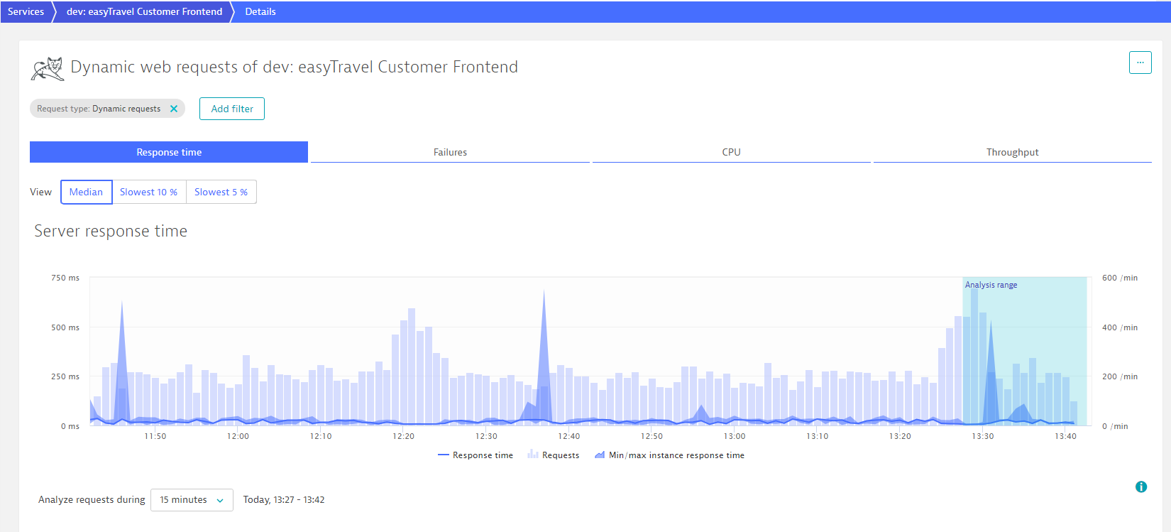
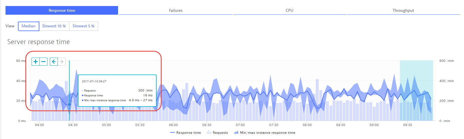
Hold your cursor over any time interval in the chart to display time-interval controls and the specific measurements for that interval, including number of Requests, Response time, Min/max instance response time, and date/time.

To adjust the time scale along the X-axis, select a different time interval from the drop list beneath the chart. Or use the +/- buttons to zoom in/out on a timeframe. The left/right arrows enable you to step forward and backward through time intervals. These buttons are visible if you move your cursor over the chart.

Outlier analysis

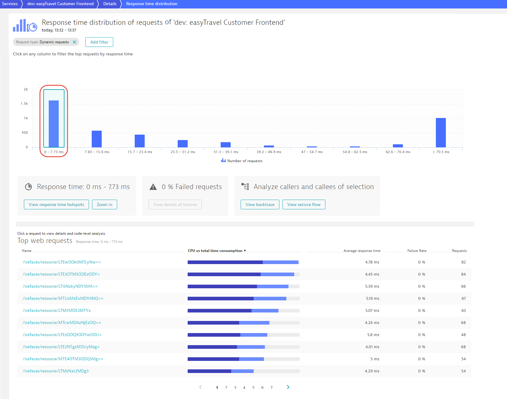
To gain a deeper understanding on how response times vary across requests during the selected period, click the Analyze outliers button to navigate to the Response time distribution page.

Click any distribution-percentile bar to view the number of requests that fall into that response time range. As you can see in the Top web requests section beneath the chart (see image below), the slowests requests (i.e., the longest response times) may take dramatically longer to execute than the fastest requests. Such outliers can have a big influence on the overall response time of a service.

You can take a closer look at the requests within each selected response time range by clicking the Zoom in button.

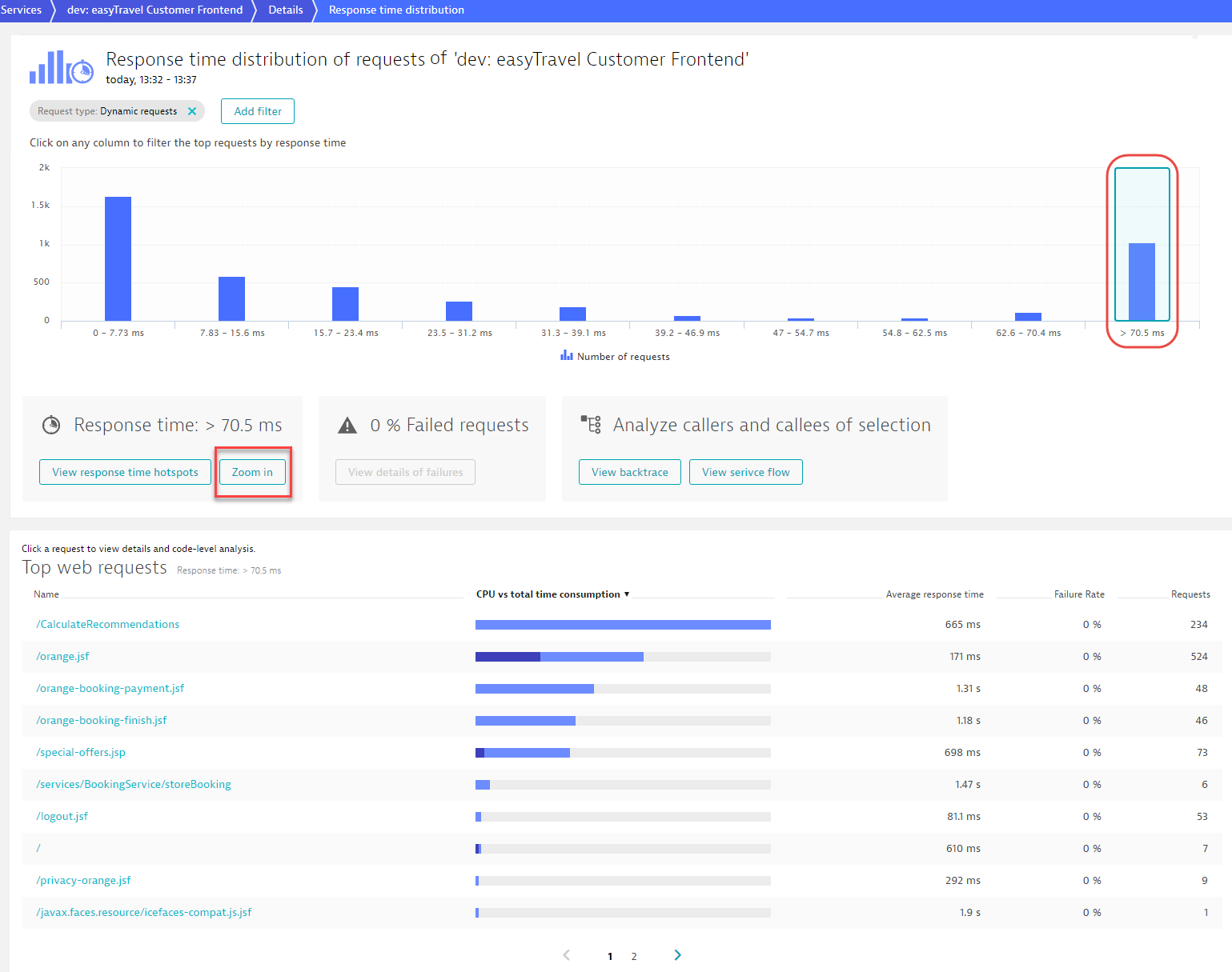
The example below shows that there are about 600 requests that have response times between 70.5 ms and 439 ms and that the orange.jsf web request contributes the most to the overall response time (491 requests during the analysis timeframe).

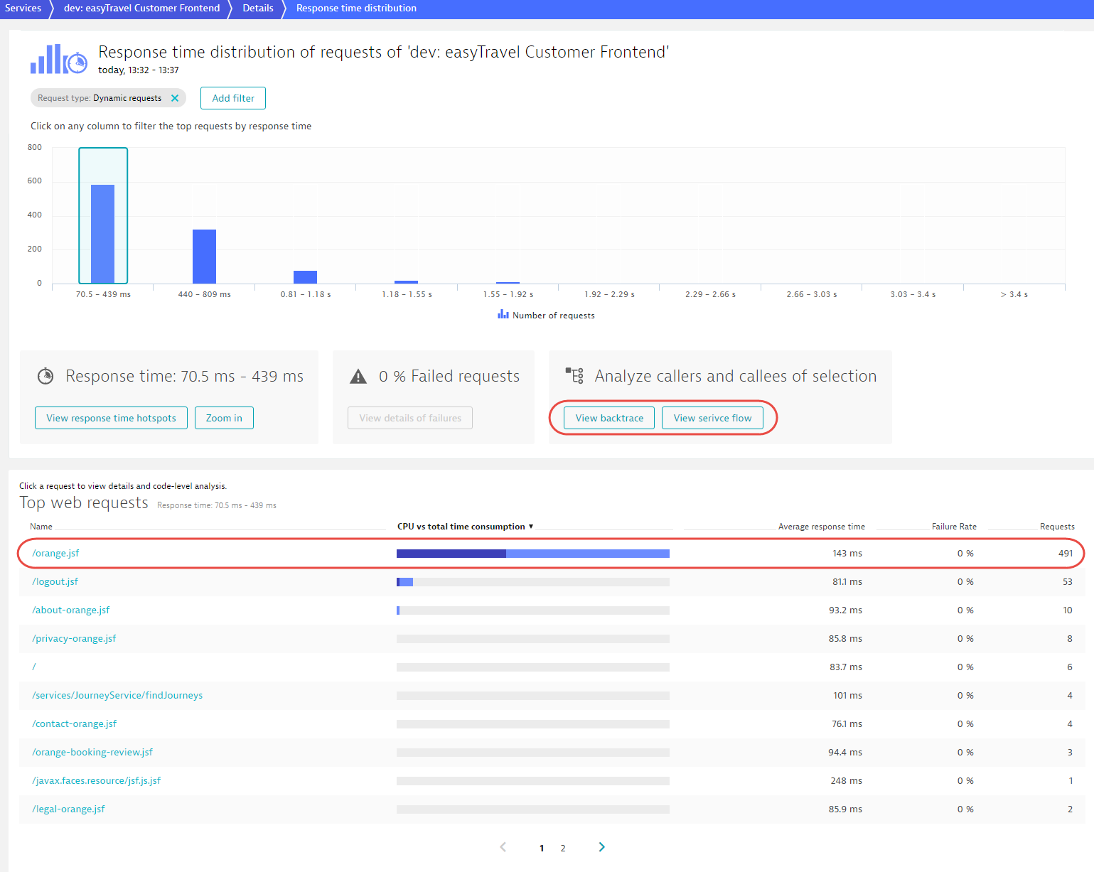
With a bar selected in the chart, click the Analyze backtrace or View service flow buttons to see where these requests fit within the overall transaction sequence.

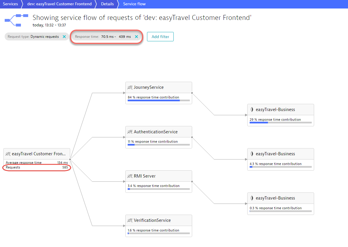
The Service flow example below shows that the requests initiated by the Customer Frontend service have response times between 70 ms and 439 ms. The JourneyService contributes the most to the response time in this example. In total, this service received 585 requests.

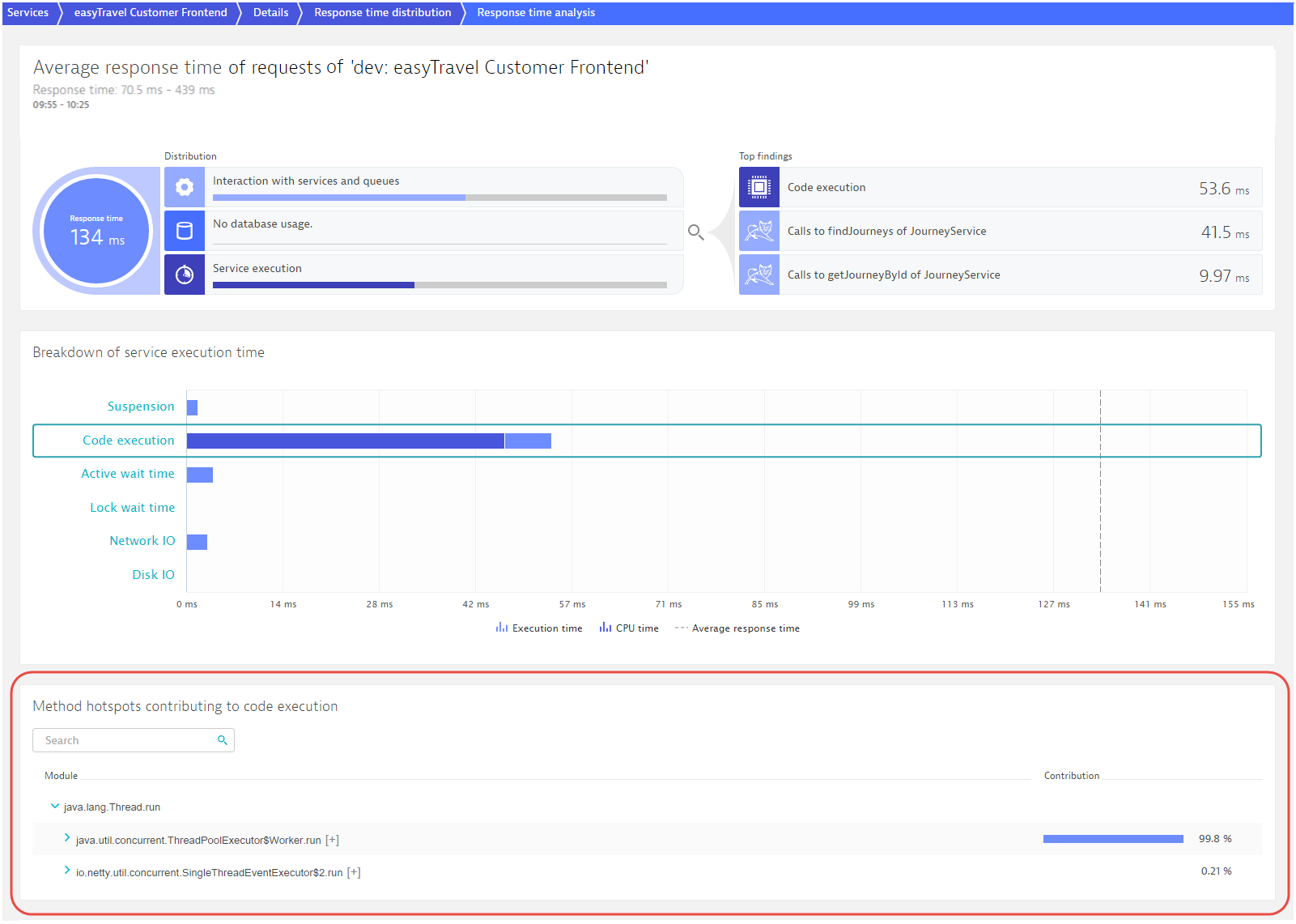
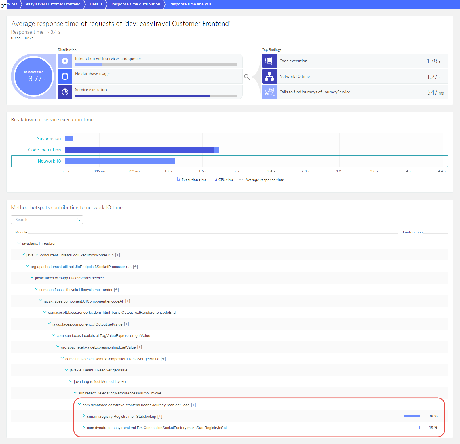
Click the View response time hotspots button to view in-depth detail related to the easyTravel Customer Frontend requests within this response time range. This gives you code-level visibility into this response-time range. Select section Service execution of the infographic to see a breakdown of the underlying service execution times. In the Breakdown of service execution time section, select Code execution to view the related Method hotspots contributing to code execution.

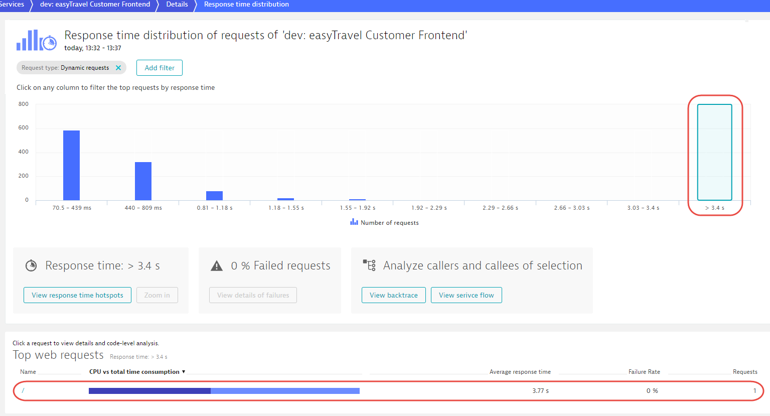
Analyze slow requests

Returning to the Response time distribution page, you can see that there are a few requests that have response times higher than 3.4 s. Clicking this column in the chart reveals further detail (see below). This last click has revealed an important insight—there is only a single request in this response time range, with a response time of 3.77 s (visible below in the Top web requests section). This single outlier has skewed the overall response time of the service. Now it's time to dig a little deeper for the root cause of this issue.

Have a look at the response time hotspot for this single request. The reason for this outlier is an RMI lookup of the JourneyBean.

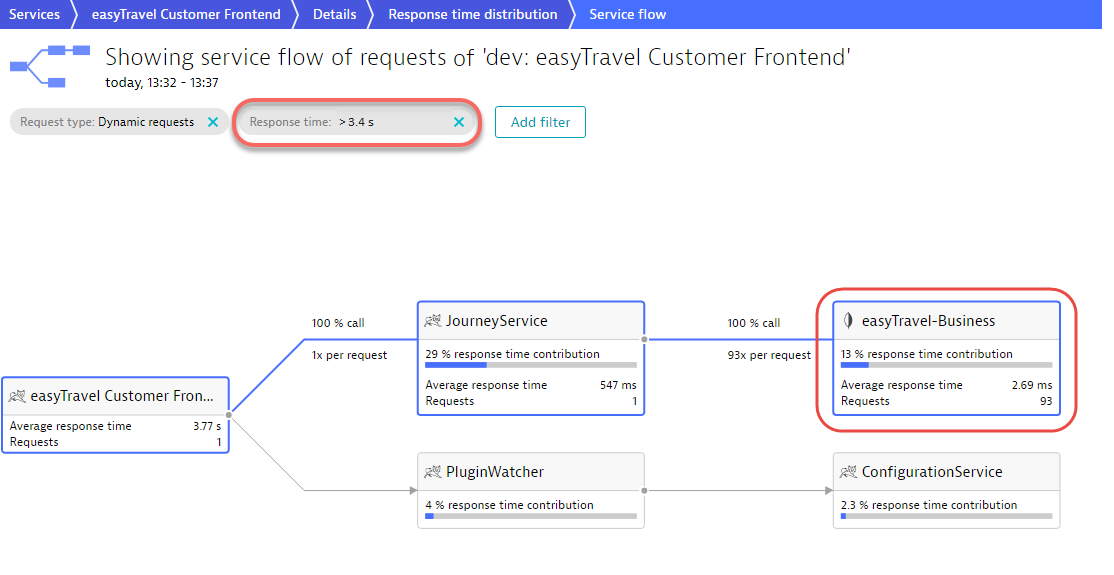
You can additionally have a look at the Service flow for this request. Service flow shows this entire transaction from end-to-end. It reveals that this single request resulted in no less than 93 database calls!

As you can see, with only a few clicks, DESK enables you to shed light on the fine-grained details of each request, down to the code level.

Correlate errors with response times

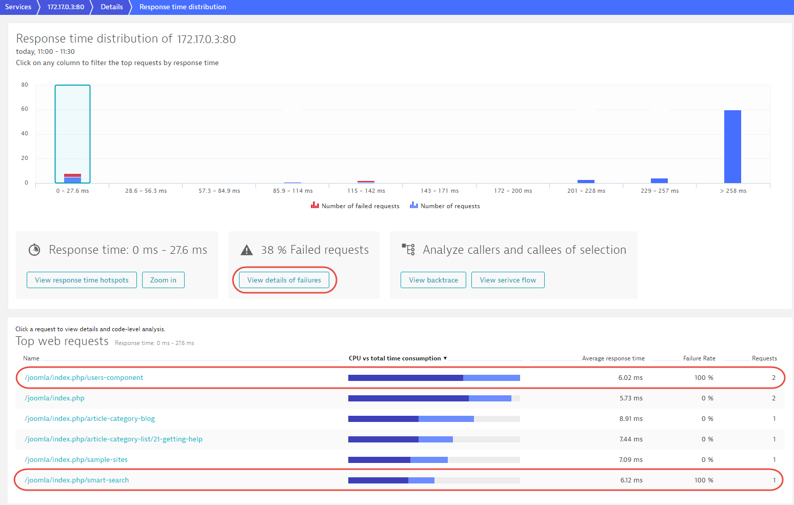
Another important aspect of response time distribution is the ability to correlate failure rate with response time. Failing requests often have particularly fast or slow response times (they either fail quickly or eventually time out). The example below shows that 38% of all requests faster than 27.6 ms are failing. A closer look at the request table reveals that these are actually two specific types of requests that always fail in this response time range. You can analyze these requests by clicking View details of failures.

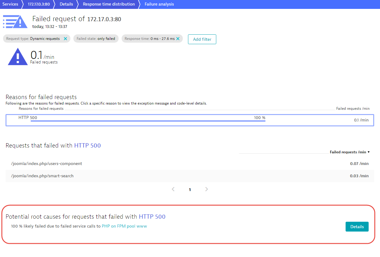
Failure analysis shows that the requests in question all fail due to an HTTP 500 error in the PHP on FPM pool www service, which can be further analyzed by clicking the Details button.

As you can see, outlier analysis, enabled by DESK response-time distribution analysis, reveals which types of requests have the largest impact on each service’s overall response time. Outlier analysis also helps you understand the correlation between specific errors and response times.